CellPhoneDB v5 new outputs
From version 5 of CellPhoneDB, there is a new output file - interaction_scores.
According to the official repository, this table corresponds to:
interaction_scores: stores the new score generated. This score ranges from 0-100.
To score interactions CellPhoneDB v5 employs the following protocol:
Exclude genes not participating in any interaction and those expressed in less than k% of cells within a given cell type.
Calculate the mean expression (G) of each gene (i) within each cell type (j).
For heteromeric proteins, aggregate the mean gene expression of each subunit (n) employing the geometric mean.
Scale mean gene/heteromer expression across cell types between 0 and 100.
Calculate the product of the scale mean expression of the interaction proteins as a proxy of the interaction relevance.
cellsign: accepts the new CellSign data.
The aim of the CellSign module is to identify activated receptors and prioritise high-confidence interactions by leveraging the activity of the downstream transcription factors (TFs). CellSign relies on a database of receptors linked to their putative downstream TFs.
ktplotspy will support these output via inclusion into the existing plot_cpdb function. We will gradually enable their functionality across the other functions, as well as with in the R package eventually.
Import libraries
[1]:
import anndata as ad
import pandas as pd
import ktplotspy as kpy
import matplotlib.pyplot as plt

from pathlib import Path
[2]:
# read in the files
# 1) .h5ad file used for performing cellphonedb
DATADIR = Path("../../data/")
adata = ad.read_h5ad(DATADIR / "ventolab_tutorial_small_adata.h5ad")

# 2) output from cellphonedb
means = pd.read_csv(DATADIR / "out_v5" / "degs_analysis_means_07_27_2023_151846.txt", sep="\t")
relevant_interactions = pd.read_csv(DATADIR / "out_v5" / "degs_analysis_relevant_interactions_07_27_2023_151846.txt", sep="\t")
interaction_scores = pd.read_csv(DATADIR / "out_v5" / "degs_analysis_interaction_scores_07_27_2023_151846.txt", sep="\t")
cellsign = pd.read_csv(DATADIR / "out_v5" / "degs_analysis_CellSign_active_interactions_07_27_2023_151846.txt", sep="\t")
[3]:
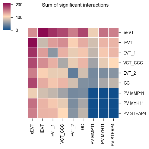
kpy.plot_cpdb_heatmap(pvals=relevant_interactions, degs_analysis=True, figsize=(5, 5), title="Sum of significant interactions")
[3]:
<seaborn.matrix.ClusterGrid at 0x77ffa58b5b20>
[4]:
kpy.plot_cpdb(
    adata=adata,
    cell_type1="PV MYH11|PV STEAP4|PV MMPP11",
    cell_type2="EVT_1|EVT_2|GC|iEVT|eEVT|VCT_CCC",
    means=means,
    pvals=relevant_interactions,
    celltype_key="cell_labels",
    genes=["TGFB2", "CSF1R"],
    figsize=(12, 3),
    title="Interactions between\nPV and trophoblast ",
    max_size=4,
    highlight_size=0.75,
    degs_analysis=True,
    standard_scale=True,
)
[4]:
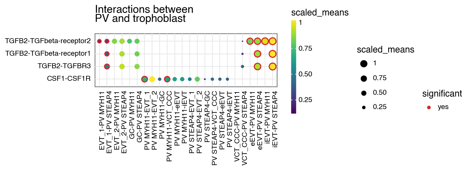
Interaction scores
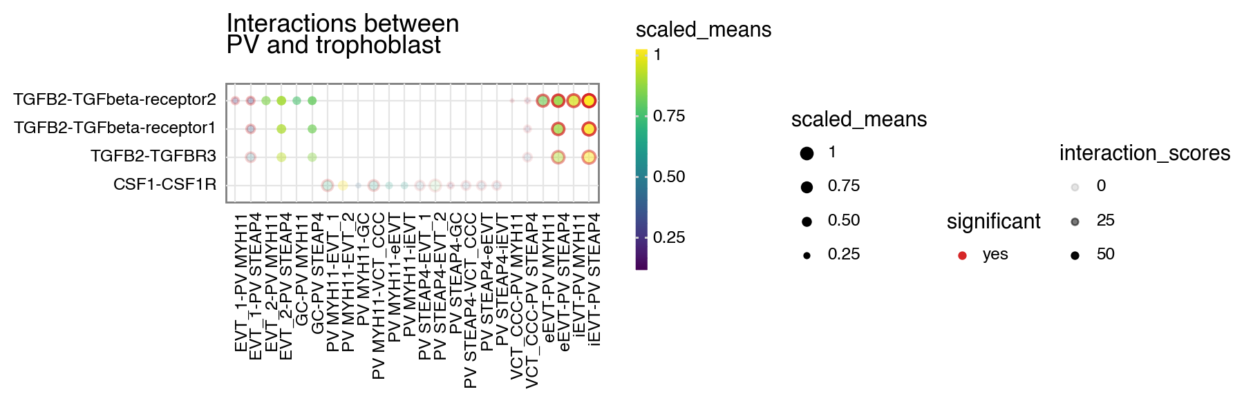
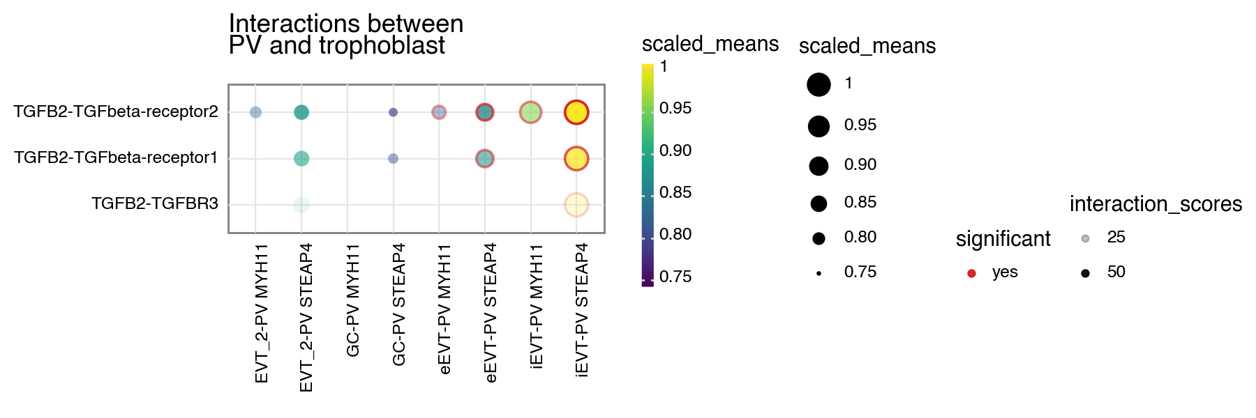
Let’s start with interaction scores. If a dataframe corresponding to the interaction_scores file is provided, you can toggle the alpha transparency of the interactions by the interaction score (interaction ranking is simply the score/100).
[5]:
kpy.plot_cpdb(
    adata=adata,
    cell_type1="PV MYH11|PV STEAP4|PV MMPP11",
    cell_type2="EVT_1|EVT_2|GC|iEVT|eEVT|VCT_CCC",
    means=means,
    pvals=relevant_interactions,
    celltype_key="cell_labels",
    genes=["TGFB2", "CSF1R"],
    figsize=(12, 3),
    title="Interactions between\nPV and trophoblast",
    max_size=3,
    highlight_size=0.75,
    degs_analysis=True,
    standard_scale=True,
    interaction_scores=interaction_scores,
    scale_alpha_by_interaction_scores=True,
)
[5]:
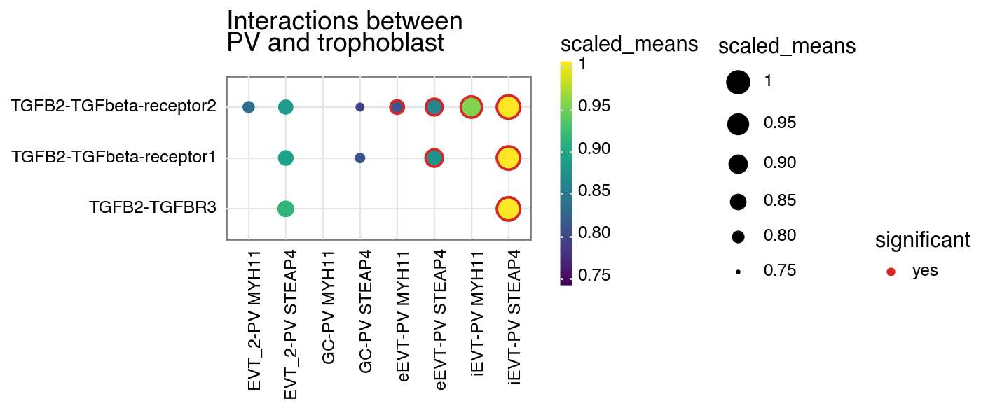
You can also specify a minimum interaction score to keep, removing all interactions lesser than this value.
[6]:
kpy.plot_cpdb(
    adata=adata,
    cell_type1="PV MYH11|PV STEAP4|PV MMPP11",
    cell_type2="EVT_1|EVT_2|GC|iEVT|eEVT|VCT_CCC",
    means=means,
    pvals=relevant_interactions,
    celltype_key="cell_labels",
    genes=["TGFB2", "CSF1R"],
    figsize=(12, 3),
    title="Interactions between\nPV and trophoblast ",
    max_size=6,
    highlight_size=0.75,
    degs_analysis=True,
    standard_scale=True,
    interaction_scores=interaction_scores,
    min_interaction_score=20,
)
[6]:
or specify both to have the alpha transparency shown too.
[7]:
kpy.plot_cpdb(
    adata=adata,
    cell_type1="PV MYH11|PV STEAP4|PV MMPP11",
    cell_type2="EVT_1|EVT_2|GC|iEVT|eEVT|VCT_CCC",
    means=means,
    pvals=relevant_interactions,
    celltype_key="cell_labels",
    genes=["TGFB2", "CSF1R"],
    figsize=(12, 3),
    title="Interactions between\nPV and trophoblast ",
    max_size=6,
    highlight_size=0.75,
    degs_analysis=True,
    standard_scale=True,
    interaction_scores=interaction_scores,
    scale_alpha_by_interaction_scores=True,
    min_interaction_score=20,
)
[7]:
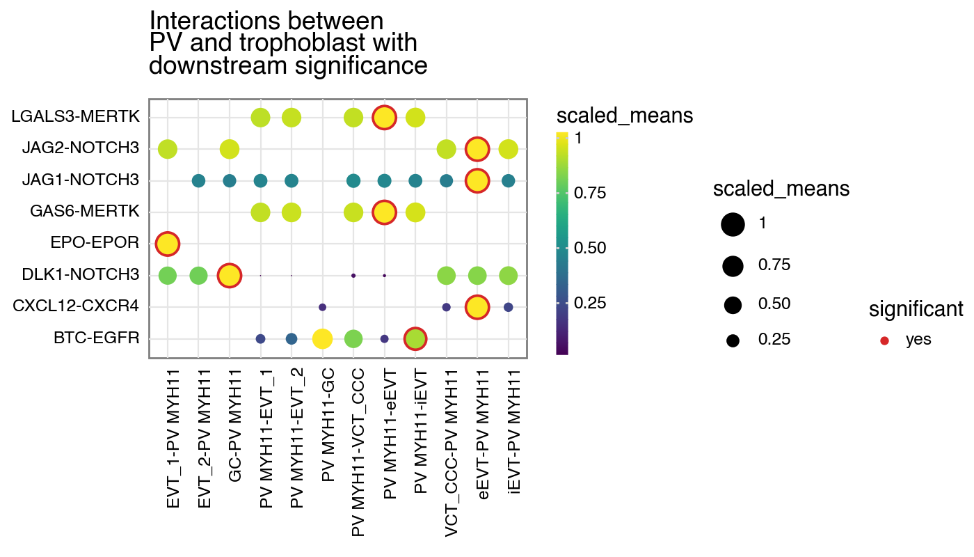
CellSign
If a dataframe corresponding to the cellsign file is provided, you can toggle the filter the interactions by the results
[8]:
kpy.plot_cpdb(
    adata=adata,
    cell_type1="PV MYH11",
    cell_type2="EVT_1|EVT_2|GC|iEVT|eEVT|VCT_CCC",
    means=means,
    pvals=relevant_interactions,
    celltype_key="cell_labels",
    figsize=(12, 4),
    title="Interactions between\nPV and trophoblast with\ndownstream significance",
    max_size=6,
    highlight_size=0.75,
    degs_analysis=True,
    standard_scale=True,
    cellsign=cellsign,
    filter_by_cellsign=True,
)
[8]:
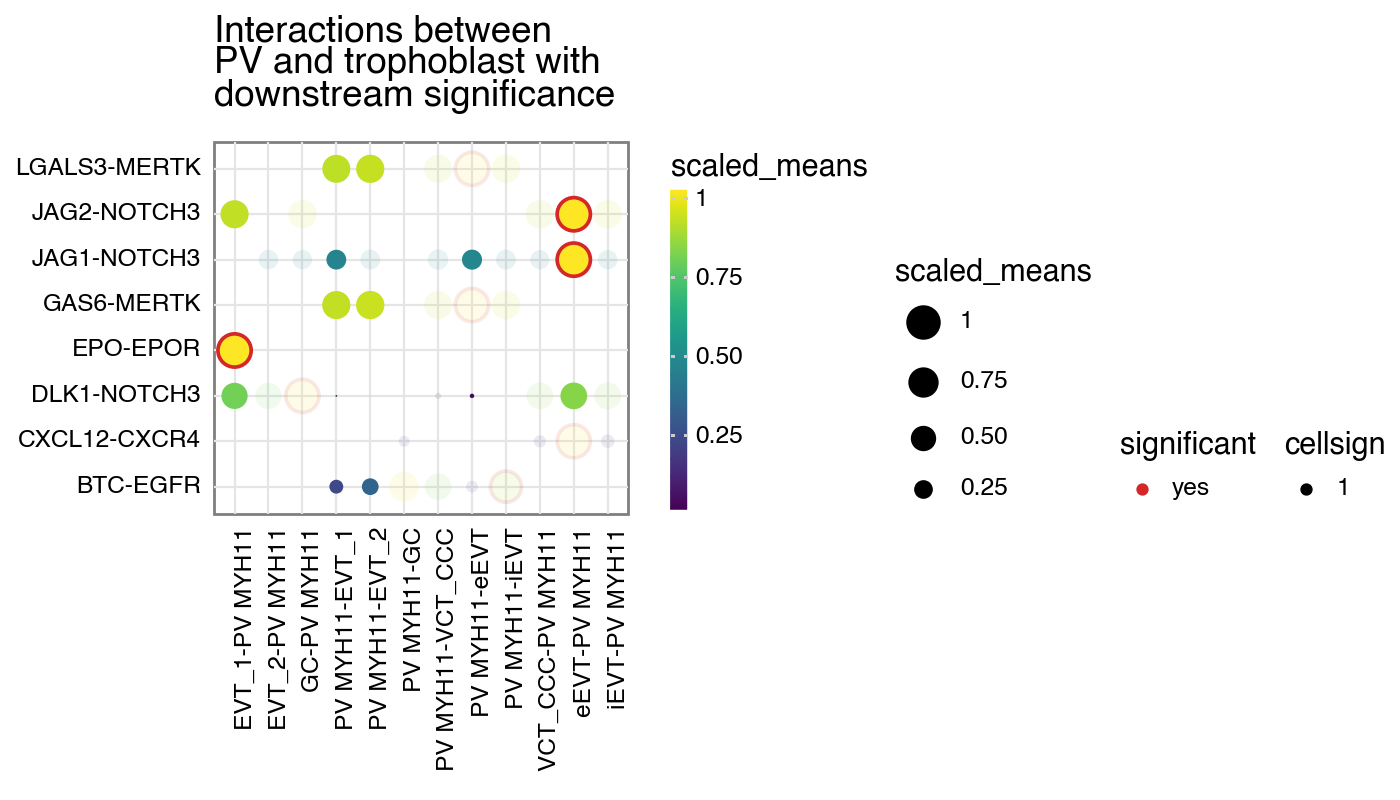
and also scale the alpha value (50% for 0 and 100% for 1).
[9]:
kpy.plot_cpdb(
    adata=adata,
    cell_type1="PV MYH11",
    cell_type2="EVT_1|EVT_2|GC|iEVT|eEVT|VCT_CCC",
    means=means,
    pvals=relevant_interactions,
    celltype_key="cell_labels",
    figsize=(12, 4),
    title="Interactions between\nPV and trophoblast with\ndownstream significance",
    max_size=6,
    highlight_size=0.75,
    degs_analysis=True,
    standard_scale=True,
    cellsign=cellsign,
    filter_by_cellsign=True,
    scale_alpha_by_cellsign=True,
)
[9]:
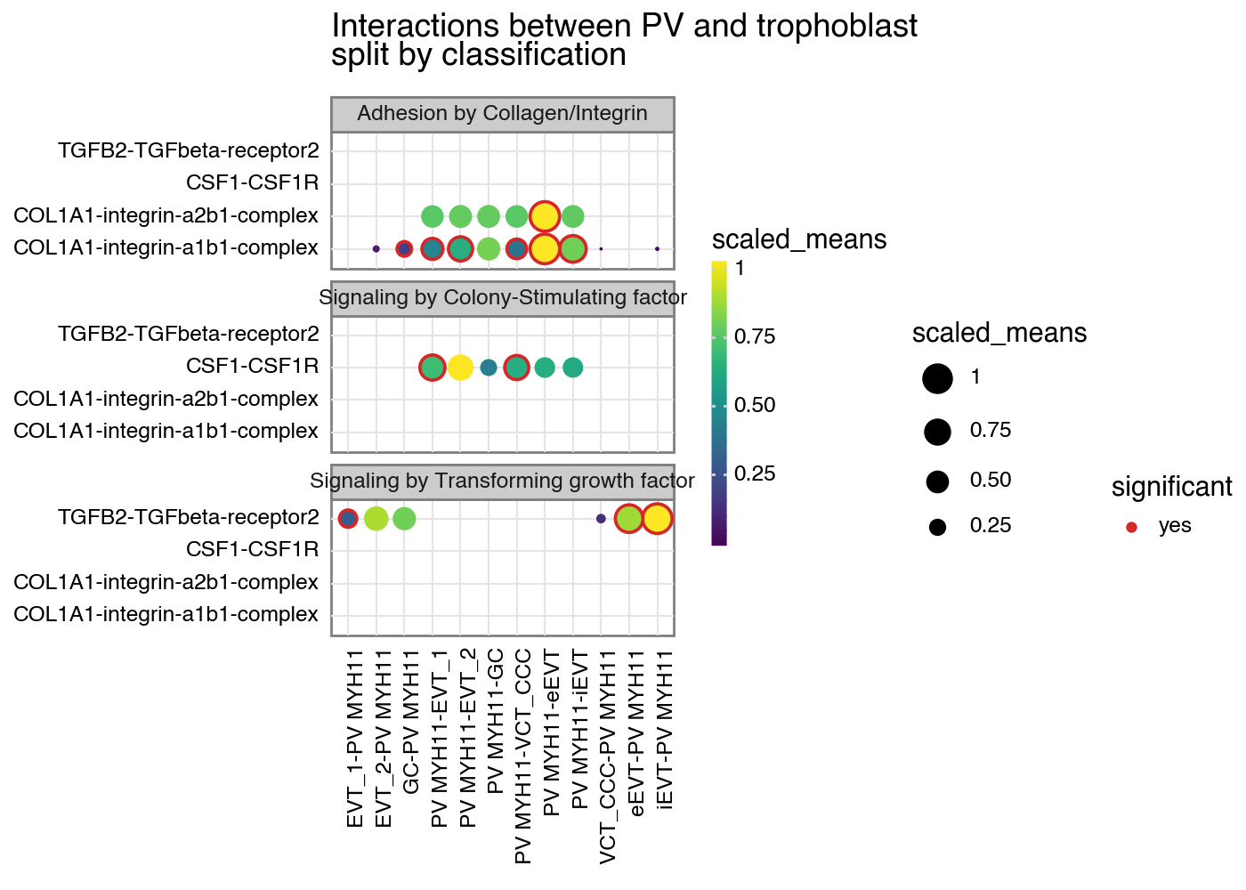
Additional plotting options
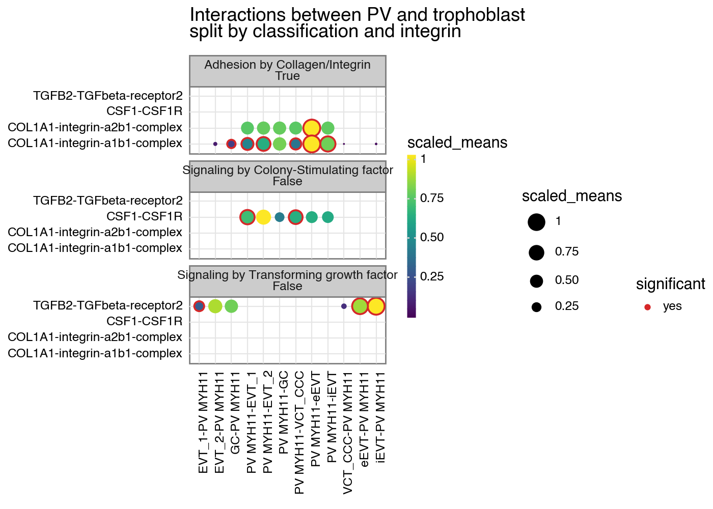
From now on, is_integrin, directionality and classification are transferred to final output table in plot_cpdb. This means you will be able to use something like facet_grid/facet_wrap to plot them!
[10]:
from plotnine import facet_wrap

p = kpy.plot_cpdb(
    adata=adata,
    cell_type1="PV MYH11",
    cell_type2="EVT_1|EVT_2|GC|iEVT|eEVT|VCT_CCC",
    means=means,
    pvals=relevant_interactions,
    celltype_key="cell_labels",
    genes=["TGFB2", "CSF1R", "COL1A1"],
    figsize=(12, 5),
    title="Interactions between PV and trophoblast\nsplit by classification",
    max_size=6,
    highlight_size=0.75,
    degs_analysis=True,
    standard_scale=True,
)
p + facet_wrap("~ classification", ncol=1)
[10]:
[11]:
p = kpy.plot_cpdb(
    adata=adata,
    cell_type1="PV MYH11",
    cell_type2="EVT_1|EVT_2|GC|iEVT|eEVT|VCT_CCC",
    means=means,
    pvals=relevant_interactions,
    celltype_key="cell_labels",
    genes=["TGFB2", "CSF1R", "COL1A1"],
    figsize=(12, 5),
    title="Interactions between PV and trophoblast\nsplit by classification and integrin",
    max_size=6,
    highlight_size=0.75,
    degs_analysis=True,
    standard_scale=True,
)
p + facet_wrap("~ classification + is_integrin", ncol=1)
[11]:
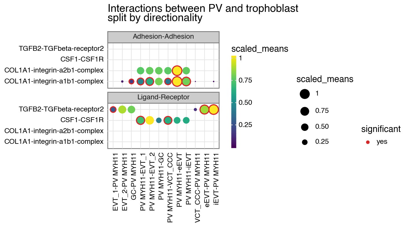
[12]:
p = kpy.plot_cpdb(
    adata=adata,
    cell_type1="PV MYH11",
    cell_type2="EVT_1|EVT_2|GC|iEVT|eEVT|VCT_CCC",
    means=means,
    pvals=relevant_interactions,
    celltype_key="cell_labels",
    genes=["TGFB2", "CSF1R", "COL1A1"],
    figsize=(12, 4),
    title="Interactions between PV and trophoblast\nsplit by directionality",
    max_size=6,
    highlight_size=0.75,
    degs_analysis=True,
    standard_scale=True,
)
p + facet_wrap("~ directionality", ncol=1)
[12]:
[ ]: